Time Constant Delay Correction in Geophysical Surveys
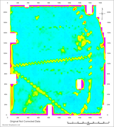
The herringbone effect is a common artifact observed on geophysical maps from electromagnetic and magnetic surveys conducted along lines traversed in opposite directions. It appears as a characteristic zigzag pattern and, in some cases, as duplicated anomalies on adjacent survey lines for a single small target.
This effect is caused by a time lag between when a measurement is taken and when it is recorded together with the sensor position.
Each instrument has its own Time Constant Delay. The magnitude of the effect is directly proportional to survey speed: the faster the system moves, the greater the distance covered during the delay, resulting in a more pronounced zigzag pattern. For this reason, the effect is particularly significant in surveys using vehicle-towed instruments. Click the images below for a larger view.
Figure 1. Data Not Corrected
Correction Method
All Geomar programs include a Time Constant Delay correction for XYZ files that contain a time stamp for each reading. The software calculates the instrument speed at each measurement point and adjusts the recorded position to compensate for the delay.
This approach is more accurate than typical “de-herringboning” algorithms because it:
preserves all original data,
does not smooth or distort anomalies,
retains even very small, high-frequency features.
Determining the Time Constant
Every sensor has a Time Constant, even if it is not specified by the manufacturer. In practice, the effective delay depends on the entire system, including the geophysical instrument and the GPS/GNSS/RTK receiver, as these components are not perfectly synchronized.
The most reliable way to determine the Time Constant for a specific system is as follows:
1. Use a dataset with survey lines crossing a linear feature (e.g., pipe, curb, or similar anomaly).
2. Generate an XYZ file and create a map (color or grayscale) showing the zigzag pattern.
3. Apply Time Constant correction in your processing software (e.g., TrackMaker, RTM, or Multi), starting with an initial value (e.g., 0.5 seconds).
4. Evaluate the result:
If the zigzag persists, increase the value (e.g., to 0.6 seconds).
Regenerate the map and reassess.
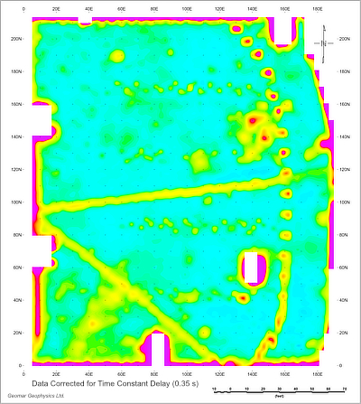
Figure 2. Data Corrected
5. Repeat the process until a satisfactory result is achieved.
Important: Always apply corrections to the original XYZ file. Do not apply corrections to already corrected data.
The result will not be mathematically perfect, but it should be sufficiently accurate for practical use.
Typical Starting Values
Based on experience, the following values are good starting points:
Geonics EM31-MK2: 0.5 – 0.75 s
Geonics EM38-MK2: 0.4 – 0.6 s
Geonics EM61-MK2: 0.3 – 0.5 s
Magnetometers: start at 0.1 s and increase in increments of 0.05 s
Important Notes
Each XYZ file must contain a time stamp for this correction to work.
Once determined, the Time Constant can be applied to future surveys using the same system, regardless of survey speed (walking or vehicle-based).
However, excessive survey speed introduces additional issues:
reduced spatial coverage,
less signal integration time,
increased noise due to mechanical vibrations
To minimize vibration-related noise, sled-mounted systems are generally preferable to wheeled trailers, especially on rough terrain.
Example
Figures 1 and 2 (click to enlarge) illustrate Time Constant Delay correction applied to Geonics EM61-MK2 data using a value of 0.35 seconds. In this case, the sensor was mounted on wheels and surveyed over a smooth asphalt surface.